Équation de diffusion à une dimension avec Scilab

1. Fonction de calcul

Ci-dessous la fonction de calcul (télécharger).

N : nombre de points
type0 : type de la condition limite en x=0, "neumann" ou "dirichlet"
lim0 : valeur de la condition limite en x=0
type1 : type de la condition limite en x=1
lim1 : valeur de la condition limite en x=1
coef : coefficients de diffusion sous la forme [[x1,D1];[x2,D2],...[1,Dk]]
S : sources, matrice colonne à n éléments
U : état initial, matrice colonne à n éléments
t : temps initial
dt : pas de temps
tf : temps final

function [U,t]=diffusion(N,type0,lim0,type1,lim1,coef,S,U,t,dt,tf)
    dx=1/(N-1)
    A=spzeros(N,N)
    B=spzeros(N,N)
    C=S*dt
    a=2*dt/dx^2
    nd=size(coef)
    nd=nd(1)
    D = zeros(N) // coefficients de diffusion
    j1=1
    for k=1:nd,
        j2 = int(coef(k,1)*N)
        d = coef(k,2)
        for j=j1:j2,
            D(j)=d
        end
        j1 = j2
    end
    for j=2:N-1, // schema de Cranck-Nicholson
        A(j,j-1)=-a*D(j)/2; B(j,j-1)=a*D(j)/2;
        A(j,j)=1+a*D(j); B(j,j)=1-a*D(j);
        A(j,j+1)=-a*D(j)/2; B(j,j+1)=a*D(j)/2;
    end;
    if type0=="dirichlet" then
        A(1,1)=1;
        A(1,2)=0;
        C(1)=lim0;
    end
    if type0=="neumann" then
        A(1,1)=-1;
        A(1,2)=1;
        C(1)=dx*lim0;
    end
    if type1=="dirichlet" then
        A(N,N-1)=0;
        A(N,N)=1;
        C(N)=lim1;
    end
    if type1=="neumann" then
        A(N,N)=1;
        A(N,N-1)=-1;
        C(N)=dx*lim1;
    end
    for k=1:nd-1,
        j = int(coef(k,1)*N)-1 // frontiere entre deux coefficients de diffusion differents
        A(j,j-1)=-D(j); A(j,j)=D(j)+D(j+1); A(j,j+1)=-D(j+1);
        B(j,j-1)=0; B(j,j)=0; B(j,j+1)=0; C(j)=0;
    end
    while t<tf // boucle de calcul
        U = lusolve(A,B*U+C);
        t = t+dt
    end
endfunction

2. Exemple : diffusion thermique dans une plaque

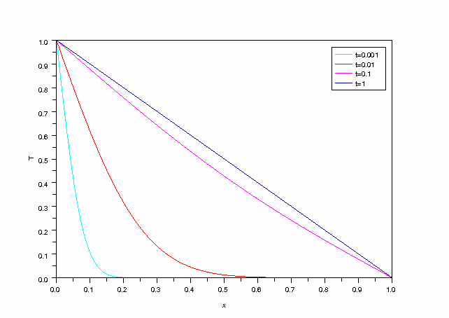
2.a. Température fixée aux bords

On considère une plaque (perpendiculaire à l'axe x) de conductivité thermique uniforme, soumise en x=0 à une température constante U=1 et en x=1 à une température constante U=0. Il n'y a aucune source thermique dans la plaque. Initialement la température est nulle sur l'intervalle [0,1].

getf('equationDiffusion1D.sci');
N=100;   
X=linspace(0,1,N).'; // vecteur colonne
U=zeros(N,1);
S=zeros(N,1);
coef=[[1,1]];

plotA=scf();
t=0;
[U1,t]=diffusion(N,'dirichlet',1,'dirichlet',0,coef,S,U,t,0.0001,0.001);
plot2d(X,U1,style=4)
[U2,t]=diffusion(N,'dirichlet',1,'dirichlet',0,coef,S,U1,t,0.001,0.01);
plot2d(X,U2,style=5)
[U3,t]=diffusion(N,'dirichlet',1,'dirichlet',0,coef,S,U2,t,0.01,0.1);
plot2d(X,U3,style=6)
[U4,t]=diffusion(N,'dirichlet',1,'dirichlet',0,coef,S,U3,t,0.1,1);
plot2d(X,U4,style=9)
plotA.children.x_label.text='x';
plotA.children.y_label.text='T';
legends(['t=0.001','t=0.01','t=0.1','t=1'],[4,5,6,9])

plotA.pdf

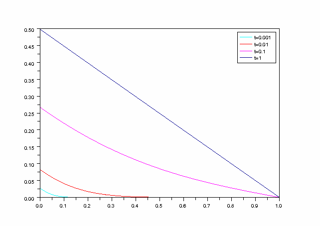
2.b. Flux thermique fixé à un bord

On reprend le cas précédent en fixant le flux thermique en x=0.

N=100;   
X=linspace(0,1,N).'; // vecteur colonne
U=zeros(N,1);
S=zeros(N,1);
coef=[[1,1]];

plotB=scf();
t=0;
[U1,t]=diffusion(N,'neumann',-0.5,'dirichlet',0,coef,S,U,t,0.0001,0.001);
plot2d(X,U1,style=4)
[U2,t]=diffusion(N,'neumann',-0.5,'dirichlet',0,coef,S,U1,t,0.001,0.01);
plot2d(X,U2,style=5)
[U3,t]=diffusion(N,'neumann',-0.5,'dirichlet',0,coef,S,U2,t,0.01,0.1);
plot2d(X,U3,style=6)
[U4,t]=diffusion(N,'neumann',-0.5,'dirichlet',0,coef,S,U3,t,0.1,1);
plot2d(X,U4,style=9)
plotA.children.x_label.text='x';
plotA.children.y_label.text='T';
legends(['t=0.001','t=0.01','t=0.1','t=1'],[4,5,6,9])

plotB.pdf

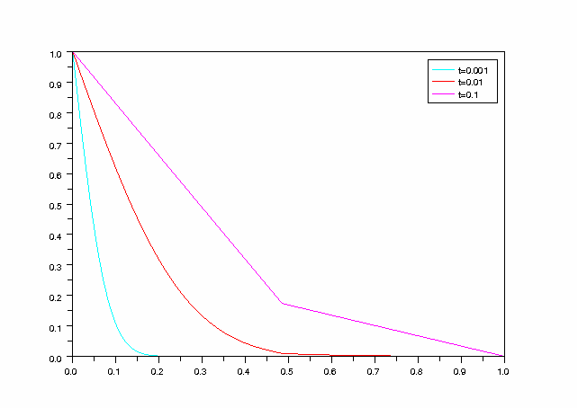
2.c. Diffusion thermique dans deux plaques

N=100;   
X=linspace(0,1,N).'; // vecteur colonne
U=zeros(N,1);
S=zeros(N,1);
coef=[[0.5,1];[1,5]];

plotC=scf();
t=0;
[U1,t]=diffusion(N,'dirichlet',1,'dirichlet',0,coef,S,U,t,0.0001,0.001);
plot2d(X,U1,style=4)
[U2,t]=diffusion(N,'dirichlet',1,'dirichlet',0,coef,S,U1,t,0.001,0.01);
plot2d(X,U2,style=5)
[U3,t]=diffusion(N,'dirichlet',1,'dirichlet',0,coef,S,U2,t,0.01,0.1);
plot2d(X,U3,style=6)
plotA.children.x_label.text='x';
plotA.children.y_label.text='T';
legends(['t=0.001','t=0.01','t=0.1'],[4,5,6])

plotC.pdf

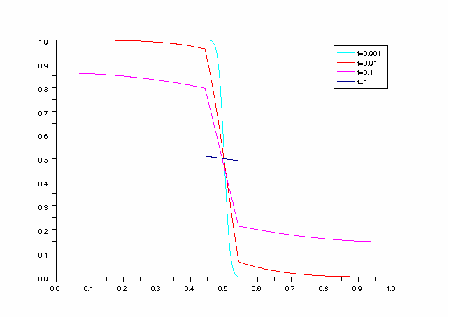
2.d. Système à trois plaques

On considère un système isolé formé de deux plaques initialement à deux températures différentes, mises en contact thermique par une troisième plaque mince de conductivité plus faible.


N=200;
U=zeros(N,1);
X=linspace(0,1,N).';
for j=1:int(N/2),
    U(j)=1;
end;
S=zeros(N,1);
coef=[[0.45,1];[0.55,0.05];[1,1]];

plotD=scf();
t=0;
[U1,t]=diffusion(N,'neumann',0,'neumann',0,coef,S,U,t,0.0001,0.001);
plot2d(X,U1,style=4)
[U2,t]=diffusion(N,'neumann',0,'neumann',0,coef,S,U1,t,0.001,0.01);
plot2d(X,U2,style=5)
[U3,t]=diffusion(N,'neumann',0,'neumann',0,coef,S,U2,t,0.01,0.1);
plot2d(X,U3,style=6)
[U4,t]=diffusion(N,'neumann',0,'neumann',0,coef,S,U3,t,0.1,1);
plot2d(X,U4,style=9)
plotA.children.x_label.text='x';
plotA.children.y_label.text='T';
legends(['t=0.001','t=0.01','t=0.1','t=1'],[4,5,6,9])

plotD.pdf