Pendule libre conservatif
1. Introduction
L'équation différentielle du mouvement d'un pendule pesant non dissipatif est :
Pour le calcul numérique, on posera une période d'oscillations harmoniques égale à 1, c'est-à-dire :
L'intégrale première (énergie mécanique) est :
2. Intégration avec Mathematica
La fonction suivante effectue l'intégration numérique pour un angle initial non nul thetaInit et une vitesse initiale nulle, pendant une durée tmax.
solution[thetaInit_,tmax_]:=Module[{sys},
    sys={theta'[t]==dtheta[t],dtheta'[t]==-4*Pi^2*Sin[theta[t]],
    theta[0]==thetaInit,dtheta[0]==0};
    NDSolve[sys,{theta,dtheta},{t,0,tmax},
            Method->{'ExplicitRungeKutta',DifferenceOrder->4},
            AccuracyGoal->5,MaxSteps->Infinity]
]
On définit une fonction pour tracer le spectre en décibel, avec en argument : la sortie de la fonction solution ci-dessus, la durée totale tmax et la période d'échantillonnage te. La transformée de Fourier discrète et son utilisation avec Mathematica sont expliquées ici.
spectre[solution_,tmax_,te_]:=Module[{n,echant,tfd,sp},
    n=tmax/te;
    echant=Table[First[theta[(k-1)*te]/.solution],{k,n}];
    tfd=Fourier[echant,FourierParameters->{-1,-1}];
    sp=Table[{(k-1)/tmax,20*Log[10,Abs[tfd[[k]]]]},{k,n}];
    ListPlot[sp,PlotRange->{{0,1/te/2},{-100,0}},Joined->True]
]
Voici un exemple pour un angle initial de 0.1 radians. On trace la trajectoire dans le plan de phase.
tmax=100;
s1=solution[0.1,tmax]
p1=ParametricPlot[{theta[t],dtheta[t]/(2*Pi)}/.s1,{t,0,10},AxesLabel->{'theta','dtheta'}]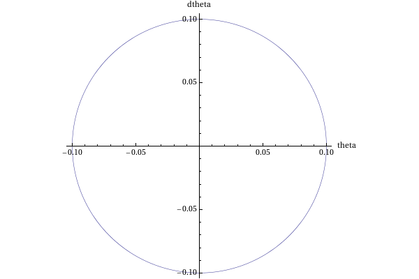 plotA.pdf
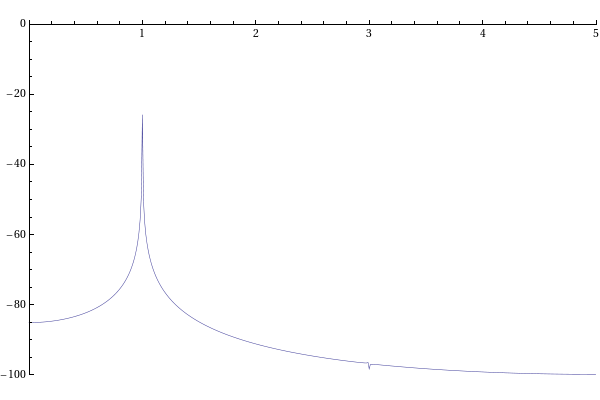
Le spectre avec une période d'échantillonnage de 0.1 :
spectre[s1,tmax,0.1]
 plotB.pdf
Un angle plus grand donne lieu a des oscillations non harmoniques :
s2=solution[Pi/2,tmax]
p2=ParametricPlot[{theta[t],dtheta[t]/(2*Pi)}/.s2,{t,0,10},AxesLabel->{'theta','dtheta'}]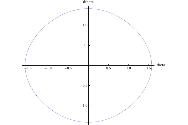 plotC.pdf
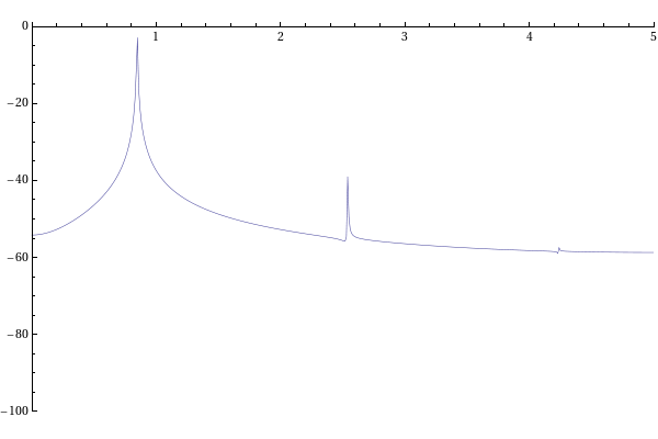
Le spectre avec une période d'échantillonnage de 0.1 :
spectre[s2,tmax,0.1]
 plotD.pdf
On remarque une baisse de la fréquence d'oscillation et l'apparition d'une harmonique de rang 3. Voyons le résutat avec un angle initial proche de π :
s3=solution[3.1,tmax]
p3=ParametricPlot[{theta[t],dtheta[t]/(2*Pi)}/.s3,{t,0,10},AxesLabel->{'theta','dtheta'}]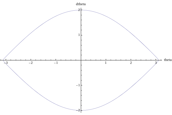 plotE.pdf
Le spectre avec une période d'échantillonnage de 0.1 :
spectre[s3,tmax,0.1]
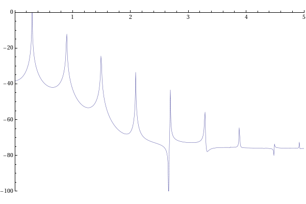 plotF.pdf
Pour ce dernier cas, traçons aussi l'énergie pour vérifier sa conservation :
Plot[0.5*dtheta[t]^2-(2*Pi)^2*Cos[theta[t]]/.s3,{t,0,tmax},PlotRange->{{0,tmax},{30,50}},
AxesLabel->{'t','Energie'}]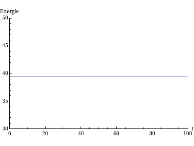 plotG.pdf
Pour finir, les trois trajectoires dans l'espace des phases :
Show[p1,p2,p3,PlotRange->{{-3,3},{-3,3}}]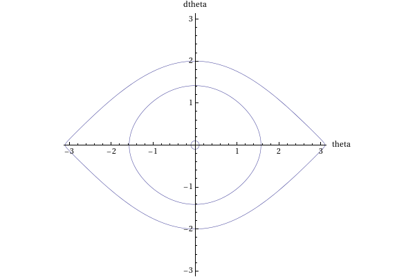 plotH.pdf
3. Intégration avec Scilab
Ci-dessous la fonction d'intégration numérique fournissant trois vecteurs (temps t, angle et dérivée y, énergie e). L'angle initial, le temps final et la période d'échantillonnage sont donnés en argument :
function [t,y,e]=solution(thetaInit,tmax,te),
    function [deriv]=systeme(t,y),
        deriv(1)=y(2),
        deriv(2)=-4*%pi^2*sin(y(1)),
    endfunction
    t=[0:te:tmax];
    tolA=1d-7;
    tolR=1d-10;
    y=ode('adams',[thetaInit;0],0,t,tolR,tolA,systeme);
    n=length(y(1,:));
    e=zeros(1,n);
    for k=1:n,
        e(k)=0.5*y(2,k)^2-4*%pi^2*cos(y(1,k));
    end;
endfunction
Fonction de tracé du spectre :
function spectre(y,tmax,te)
    tfd=fft(y);
    n=length(y);
    sp=zeros(1,n);
    f=zeros(1,n);
    for k=1:n,
        sp(k)=20*log10(abs(tfd(k)));
        f(k)=(k-1)/tmax;
    end;
    plot2d(f,sp,rect=[0,-50,1/te/2,100]);
endfunction
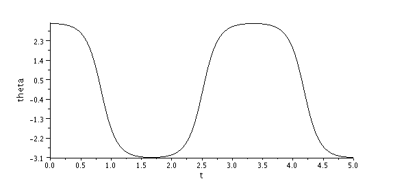
Exemple pour un angle initial de 3.1 radians :
tmax=100;
[t,y1,e1]=solution(3.1,tmax,0.01);
plotK=scf();
plot2d(t,y1(1,:),rect=[0,-%pi,5,%pi]);
xtitle('','t','theta');
 plotK.pdf
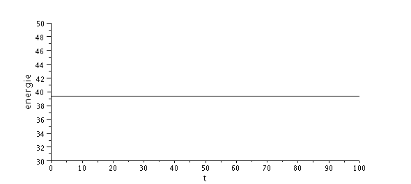
plotL=scf();
plot2d(t,e1,rect=[0,30,tmax,50]);
xtitle('','t','energie');
 plotL.pdf
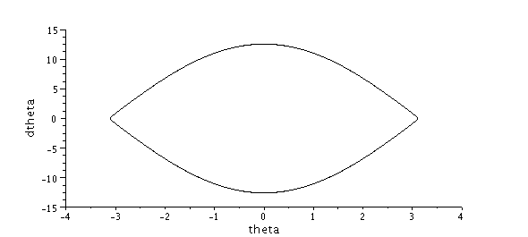
plotI=scf();
plot2d(y1(1,:),y1(2,:))
xtitle('','theta','dtheta');
 plotI.pdf
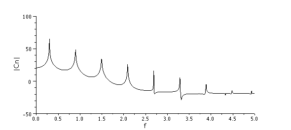
[t,y1,e1]=solution(3.1,tmax,0.1);
plotJ=scf();
spectre(y1(1,:),tmax,0.1);
xtitle('','f','|Cn|');
 plotJ.pdf